


CPG demand forecasting: A guide to getting started
Inventory distortion costs the global retail economy roughly $1.73 trillion annually. For CPG brands, this number represents a constant tension between costly overstocks and facing stockouts on the shelf. The difference between profit and waste often comes down to the quality of your demand signal. While teams have historically relied on shipment history to predict the future, this approach ignores the reality of what is actually happening in stores. Effective forecasting requires moving beyond what you shipped to capturing consumer buying signals in real-time.
Key takeaways:
- Shipment data is a lagging indicator that masks true consumer demand due to supply chain buffers and order timing.
- Separating baseline demand from promotional lift is necessary to prevent historical data from contaminating future predictions.
- On-Shelf Availability (OSA) is a critical metric for understanding how often products are actually available for purchase when consumers want them.
- Velocity (same-store sales velocity) serves as a north star metric by revealing true demand patterns beyond distribution expansion.
- Real-time point-of-sale (POS) data provides the granularity needed to move from reactive planning to proactive demand sensing.
Relying on shipment data alone ignores the reality of what’s actually happening in stores. Effective forecasting requires moving beyond what you shipped to capturing consumer buying signals in real-time.
The problem with shipment-based forecasting
Many CPG manufacturers begin their forecasting journey by analyzing historical shipment data. While this data is easily accessible internally, it represents constrained demand. Shipments reflect what you sent to a retailer, which is often limited by inventory availability, logistics constraints, or production capacity. It rarely mirrors exactly what the consumer wanted to buy.
Relying solely on shipments creates a disconnect known as the bullwhip effect. Small fluctuations in consumer demand at the shelf cause increasingly larger variances in orders as you move up the supply chain. A retailer might delay ordering for two weeks to burn down backstock, then place a massive restocking order. If your forecast interprets that large order as a spike in consumer interest, you will overproduce.
To fix this, you must shift focus to True Demand. This is an estimate of what you optimally could sell if product availability were unlimited. The closest proxy for this in the real world is point-of-sale (POS) data, or consumption data. Analyzing daily sales at the store-level removes the noise of warehouse buffering and provides a clearer signal of actual consumption trends.
Reduce out-of-stocks (OOS) with real-time data
Establishing the right retail data hierarchy
Getting started with advanced forecasting requires organizing your data effectively. A forecast is only as good as its granularity. Broad national averages, such as what’s typically available in syndicated market reports, hide regional variations, and monthly aggregates miss crucial weekly trends.
You can effectively define your hierarchy across three dimensions:
- Product: Drill down to the SKU-level rather than just the brand or category-level.
- Location: Differentiate between national, distribution center (DC), and individual store levels.
- Time: Move from monthly buckets to weekly or daily reports.
High-level forecasts often look accurate because errors cancel each other out. You might be over-forecasted in the Northeast and under-forecasted in the South, making the national number look perfect while you lose sales in both regions. Breaking data down allows you to identify specific problem areas.
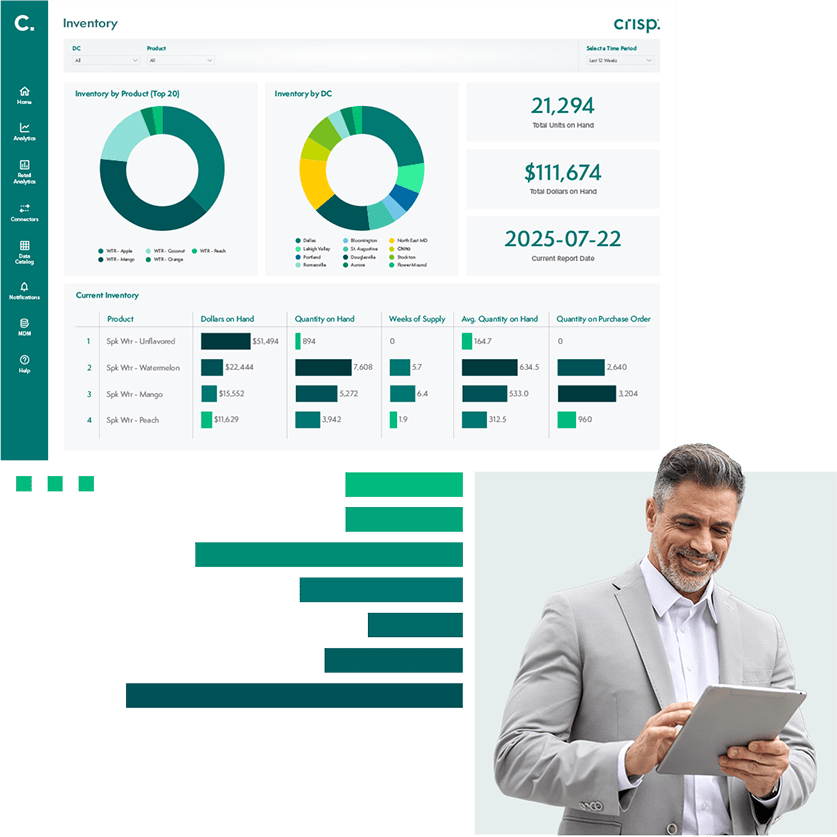
Teams should also integrate inventory data into this hierarchy. Knowing your real-time inventory levels at retailer DCs and stores helps you understand if a dip in sales is due to a lack of demand or a lack of stock. If sales drop because the product wasn’t on the shelf, your forecast model needs to know that to avoid projecting that dip into the future.
Knowing your real-time inventory levels at retailer DCs and stores helps you understand if a dip in sales is due to a lack of demand or a lack of stock.
Separating baseline demand from lift
A common pitfall in CPG forecasting is treating all historical volume as equal. If you sold 10,000 units last July, a simple model might predict 10,000 units for this July. However, if 4,000 of those units were driven by a BOGO sales promotion, your baseline demand was only 6,000.
You can decompose your history into two distinct streams:
- Base demand: The recurring volume you sell without special incentives.
- Incremental lift: The additional volume driven by promotions, temporary price cuts, or specific events.
Isolating the baseline-demand forecast enables you to see the true health of your brand. If your baseline is declining while total sales are flat, you are becoming overly reliant on promotions to move volume.
Once you have a clean baseline, you can layer promotional effects back in. This requires maintaining a rigorous calendar of past and future trade events. When you plan a promotion for the upcoming quarter, you apply a lift coefficient based on how similar promotions performed in the past. This separation prevents “unusual events” from contaminating your long-term baseline.
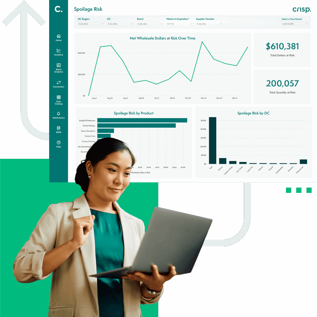
Reduce waste and boost operational efficiency
If you sold 10,000 units last July, a simple model might predict 10,000 units for this July. However, if 4,000 of those units were driven by a BOGO sales promotion, your baseline demand was only 6,000.
Focusing on the right metrics: OSA and Velocity
How you measure success dictates how your team behaves. For CPG forecasting, two metrics stand out as particularly actionable: On-Shelf Availability (OSA) and Velocity. These metrics directly connect demand forecasting to the outcomes that matter most – products being available when consumers want to buy them and understanding true demand patterns.
On-Shelf Availability (OSA)
On-Shelf Availability, also known as Walk-In Purchasability (WIP%), measures how often products are actually available for purchase when consumers want them. A perfect forecast is worthless if the product isn’t on the shelf when shoppers are looking for it. OSA provides a direct line of sight into whether your forecasting and supply chain execution are working together to meet consumer demand. Low OSA despite accurate forecasting points to fulfillment or logistics gaps that need to be addressed.
Velocity
Velocity, specifically same-store sales velocity, serves as a north star metric for understanding true demand patterns. Unlike total sales, which can be distorted by distribution expansion or contraction, velocity reveals how well products are selling in established locations. This metric is critical for forecasting because it isolates organic demand growth from the noise of changing distribution. When velocity increases, you know consumer demand is genuinely strengthening, giving you confidence to forecast higher volumes.
Together, OSA and Velocity create a complete picture: Velocity tells you what the underlying demand trend is, while OSA tells you whether you’re actually capturing that demand. If velocity is strong but OSA is low, you’re leaving money on the table. If OSA is high but velocity is declining, you may be overstocked relative to actual demand.
By focusing on these two metrics, teams can align their forecasting efforts with the business outcomes that drive revenue and profitability: keeping products available for purchase and accurately understanding consumer demand independent of distribution changes.
OSA provides a direct line of sight into whether your forecasting and supply chain execution are working together to meet consumer demand.
Moving toward demand sensing
Traditional demand planning relies on history to predict the future. Demand sensing uses near-real-time data to adjust the forecast in the short term. This is critical for fast-moving CPG categories where trends shift rapidly.
Demand sensing incorporates POS data and order signals to detect deviations from the plan immediately. If a social media trend causes a spike in consumption on a Tuesday, demand sensing picks up the signal by Wednesday, allowing supply chain teams to expedite replenishment before the weekend out-of-stocks occur.
Implementing this requires access to timely data. Relying on monthly syndicated reports or messy retailer portals creates a latency that makes sensing impossible. You need a continuous flow of data from retailers to your planning tools.
With the emergence of Agentic AI, CPGs can now assimilate hundreds of analyses of past promotions and current conditions to forecast both true demand for upcoming events, such as promotions, new product launches, or price changes, and achieve uplifts, based on historic execution limitations. However, the accuracy of AI-powered forecasting depends entirely on the quality and consistency of the underlying data foundation. Clean, granular, real-time data is essential for training AI models that can detect patterns and predict demand shifts with precision.This is where platforms like Crisp provide value. By automating the ingestion and normalization of daily sales and inventory data from 60+ retailers and distributors, Crisp creates a consistent signal that can feed directly into forecasting models. Instead of spending hours wrangling spreadsheets and extracting meaningful insights, teams can focus on analyzing clean, daily trends directly tied to forecasting accuracy.

Five AI strategies for retail supply chains
Using case studies to benchmark success
Brands like Safe Catch use daily sales and inventory visibility to identify distribution gaps and out-of-stocks early. By acting on store-level signals instead of delayed reports, Safe Catch recovered over $1M in lost sales tied directly to availability issues– strengthening retailer relationships while improving on-shelf performance.
Accurate forecasting is rarely about having the most complex algorithms. Today’s leading CPGs find success with the cleanest, most granular data and a process that allows their teams to react to it.
Next steps for implementation
Improving your forecasting capability is an iterative process. You can’t overhaul your entire portfolio overnight.
Start by identifying your “A-items” – the high-volume SKUs that drive the majority of your revenue. Audit the data you currently use to forecast them. Are you using shipments or consumption? Do you have a clear view of inventory in the channel?
Next, establish a simple baseline forecast for these items, such as leveraging a moving average. Measure the error of this simple forecast against your actual sales for three months. This gives you a benchmark.
Once you have a benchmark, begin layering in causal factors like promotions and distribution changes. Measure if these additions improve your forecast accuracy or degrade it. By treating forecasting as a series of experiments rather than a rigid yearly exercise, you build a resilient system capable of handling market volatility.
FAQs about CPG demand forecasting
-
What is the difference between demand planning and demand forecasting?
Demand forecasting is the analytical process of estimating future consumer demand using data and statistical models. Demand planning is the broader management process that uses those forecasts to align inventory, production, and sales strategies to meet business goals. The forecast is the input; the plan is the execution strategy.
-
How does demand sensing differ from traditional forecasting?
Demand sensing focuses on the short-term horizon (days or weeks) using real-time signals like POS data, weather, and open orders to adjust predictions rapidly. Traditional forecasting typically looks at longer horizons (months or quarters) based primarily on historical shipment data and seasonal patterns. Sensing captures immediate market shifts that traditional methods miss.
-
Why are OSA and Velocity important metrics for CPG forecasting?
On-Shelf Availability (OSA) measures whether products are actually available when consumers want to buy them, directly connecting forecasting accuracy to revenue capture. Velocity (same-store sales velocity) reveals true demand patterns independent of distribution changes, helping you distinguish between organic growth and expansion-driven sales increases. Together, these metrics ensure that forecasts translate into products being on shelves when needed and accurately reflect genuine consumer demand.
-
How should new product launches be forecasted without historical data?
New products should be forecasted using “attribute-based” modeling, where you analyze the performance of similar existing products (look-alikes) with comparable price points, packaging, or category placement. Teams often create a range of scenarios – conservative, expected, and optimistic – and refine the forecast weekly as early consumption data becomes available.
-
What is the impact of promotions on demand forecasting accuracy?
Promotions introduce significant volatility that can distort baseline accuracy if not isolated. They require specific “lift coefficients” to predict the incremental volume above baseline sales. Failing to separate promotional volume from regular sales history can artificially inflate future baseline predictions, leading to overstocking once the promotion ends.
-
How would you forecast demand at the SKU level given trends and seasonalities?
Forecasting demand at the SKU level starts with clean, daily POS and inventory data by store (retail demand forecasting — getting started), since models trained on stockout-suppressed zeros will systematically underforecast. Crisp pulls that data directly from retailer portals and standardizes it, while AI Master Data keeps product hierarchies consistent so forecasts reconcile cleanly across DCs and banners. From there, segment SKUs by velocity, apply seasonal methods to predictable movers and intermittent-demand approaches to slow ones, and build probabilistic outputs that tie directly to service-level targets. Crisp’s forecasting and order automation rebuilds models per SKU, per store, daily (Smart Replenishment), factoring in holidays, weather, and local events.
Get insights from your retail data
Crisp connects, normalizes, and analyzes disparate retail data sources, providing CPG brands with up-to-date, actionable insights to grow their business.